This module introduces how non-@ud mathematics are instrumented in Hoon. It may be considered optional and skipped if you are speedrunning Hoon School.
All of the math we've done until this point relied on unsigned integers: there was no negative value possible, and there were no numbers with a fractional part. How can we work with mathematics that require more than just bare unsigned integers?
@u unsigned integers (whether @ud decimal, @ux hexadecimal, etc.) simply count upwards by binary place value from zero. However, if we apply a different interpretive rule to the resulting value, we can treat the integer (in memory) as if it corresponded to a different real value, such as a negative number↗ or a number with a fractional part↗. Auras make this straightforward to explore:
> `@ud`1.000.0001.000.000> `@ux`1.000.0000xf.4240> `@ub`1.000.0000b1111.0100.0010.0100.0000> `@sd`1.000.000--500.000> `@rs`1.000.000.1.401298e-39> `@rh`1.000.000.~~3.125> `@t`1.000.000'@B\0f'
How can we actually treat other modes of interpreting numbers as mathematical quantities correctly? That's the subject of this lesson.
(Ultimately, we are using a concept called Gödel numbering↗ to justify mapping some data to a particular representation as a unique integer.)
Floating-Point Mathematics
A number with a fractional part is called a “floating-point number” in computer science. This derives from its solution to the problem of representing the part less than one.
Consider for a moment how you would represent a regular decimal fraction if you only had integers available. You would probably adopt one of three strategies:
- Rational numbers. Track whole-number ratios like fractions. Thus , thence the pair
(5, 4). Two numbers have to be tracked: the numerator and the denominator. - Fixed-point. Track the value in smaller fixed units (such as thousandths). By defining the base unit to be , may be written . One number needs to be tracked: the value in terms of the scale. (This is equivalent to rational numbers with only a fixed denominator allowed.)
- Floating-point. Track the value at adjustable scale. In this case, one needs to represent as something like . Two numbers have to be tracked: the significand () and the exponent ().
Most systems use floating-point mathematics to solve this problem. For instance, single-precision floating-point mathematics designate one bit for the sign, eight bits for the exponent (which has 127 subtracted from it), and twenty-three bits for the significand.

This number, 0b11.1110.0010.0000.0000.0000.0000.0000, is converted to decimal as .
(If you want to explore the bitwise representation of values, this tool↗ allows you to tweak values directly and see the results.)
Hoon Operations
Hoon utilizes the IEEE 754↗ implementation of floating-point math for four bitwidth representations.
| Aura | Meaning | Example |
|---|---|---|
@r | Floating-point value | |
@rh | Half-precision 16-bit mathematics | .~~4.5 |
@rs | Single-precision 32-bit mathematics | .4.5 |
@rd | Double-precision 64-bit mathematics | .~4.5 |
@rq | Quadruple-precision 128-bit mathematics | .~~~4.5 |
There are also a few molds which can represent the separate values of the FP representation. These are used internally but mostly don't appear in userspace code.
As the arms for the four @r auras are identical within their appropriate core, we will use @rs single-precision floating-point mathematics to demonstrate all operations.
Conversion to and from other auras
Any @ud unsigned decimal integer can be directly cast as an @rs.
> `@ud`.11.065.353.216
However, as you can see here, the conversion is not “correct” for the perceived values. Examining the @ux hexadecimal and @ub binary representation shows why:
> `@ux`.10x3f80.0000> `@ub`.10b11.1111.1000.0000.0000.0000.0000.0000
If you refer back to the 32-bit floating-point example above, you'll see why: to represent one exactly, we have to use and thus 0b11.1111.1000.0000.0000.0000.0000.0000.
So to carry out this conversion from @ud to @rs correctly, we should use the ++sun:rs arm.
> (sun:rs 1).1
To go the other way requires us to use an algorithm for converting an arbitrary number with a fractional part back into @ud unsigned integers. The ++fl named tuple representation serves this purpose, and uses the Dragon4 algorithm↗ to accomplish the conversion:
> (drg:rs .1)[%d s=%.y e=--0 a=1]> (drg:rs .3.1415926535)[%d s=%.y e=-7 a=31.415.927]> (drg:rs .1000)[%d s=%.y e=--3 a=1]
It's up to you to decide how to handle this result, however! Perhaps a better option for many cases is to round the answer to an @s integer with ++toi:rs:
> (toi:rs .3.1415926535)[~ --3]
(@s signed integer math is discussed below.)
Floating-point specific operations
As with aura conversion, the standard mathematical operators don't work for @rs:
> (add .1 1)1.065.353.217> `@rs`(add .1 1).1.0000001
The ++rs core defines a set of @rs-affiliated operations which should be used instead:
> (add:rs .1 .1).2
This includes:
- ++add:rs, addition
- ++sub:rs, subtraction
- ++mul:rs, multiplication
- ++div:rs, division
- ++gth:rs, greater than
- ++gte:rs, greater than or equal to
- ++lth:rs, less than
- ++lte:rs, less than or equal to
- ++equ:rs, check equality (but not nearness!)
- ++sqt:rs, square root
Exercise: ++is-close
The ++equ:rs arm checks for complete equality of two values. The downside of this arm is that it doesn't find very close values:
> (equ:rs .1 .1)%.y> (equ:rs .1 .0.9999999)%.n
Produce an arm which check for two values to be close to each other by an absolute amount. It should accept three values:
a,b, andatol. It should return the result of the following comparison:
Tutorial: Length Converter
- Write a generator to take a
@tasinput measurement unit of length, a@rsvalue, and a@tasoutput unit to which we will convert the input measurement. For instance, this generator could convert a number of imperial feet to metric decameters.
/gen/convert-length.hoon
Click to expand
|= [fr-meas=@tas num=@rs to-meas=@tas]=<^- @rs?. (check fr-meas to-meas)~|("Invalid Measures" !!)(output (meters fr-meas num) to-meas)::|%+$ allowed ?(%inch %foot %yard %furlong %chain %link %rod %fathom %shackle %cable %nautical-mile %hand %span %cubit %ell %bolt %league %megalithic-yard %smoot %barleycorn %poppy-seed %atto %femto %pico %nano %micro %milli %centi %deci %meter %deca %hecto %kilo %mega %giga %tera %peta %exa)::++ check|= [fr-meas=@tas to-meas=@tas]&(?=(allowed fr-meas) ?=(allowed to-meas))::++ meters|= [in=@tas value=@rs]=/ factor-one(~(got by convert-to-map) in)(mul:rs value factor-one)::++ output|= [in=@rs out=@tas]?: =(out %meter)in(div:rs in (~(got by convert-to-map) out))::++ convert-to-map^- (map @tas @rs)%- malt^- (list [@tas @rs]):~ :- %atto .1e-18:- %femto .1e-15:- %pico .1e-12:- %nano .1e-8:- %micro .1e-6:- %milli .1e-3:- %poppy-seed .2.212e-2:- %barleycorn .8.47e-2:- %centi .1e-2:- %inch .2.54e-2:- %deci .1e-1:- %hand .1.016e-1:- %link .2.012e-1:- %span .2.228e-1:- %foot .3.048e-1:- %cubit .4.472e-1:- %megalithic-yard .8.291e-1:- %yard .9.145e-1:- %ell .1.143:- %smoot .1.7:- %fathom .1.83:- %rod .5.03:- %deca .1e1:- %chain .2.012e1:- %shackle .2.743e1:- %bolt .3.658e1:- %hecto .1e2:- %cable .1.8532e2:- %furlong .2.0117e2:- %kilo .1e3:- %mile .1.609e3:- %nautical-mile .1.850e3:- %league .4.830e3:- %mega .1e6:- %giga .1e8:- %tera .1e12:- %peta .1e15:- %exa .1e18:- %meter .1==--
This program shows several interesting aspects, which we've covered before but highlight here:
- Meters form the standard unit of length.
~|sigbar produces an error message in case of a bad input.+$lusbuc is a type constructor arm, here for a type union over units of length.
Exercise: Measurement Converter
- Add to this generator the ability to convert some other measurement (volume, mass, force, or another of your choosing).
- Add an argument to the cell required by the gate that indicates whether the measurements are distance or your new measurement.
- Enforce strictly that the
fr-measandto-measvalues are either lengths or your new type. - Create a new map of conversion values to handle your new measurement conversion method.
- Convert the functionality into a library.
++rs as a Door
What is ++rs? It's a door with 21 arms:
> rs<21|ezj [r=?(%d %n %u %z) <51.njr 139.oyl 33.uof 1.pnw %138>]>
The battery of this core, pretty-printed as 21|ezj, has 21 arms that define functions specifically for @rs atoms. One of these arms is named ++add; it's a different add from the standard one we've been using for vanilla atoms, and thus the one we used above. When you invoke add:rs instead of just add in a function call, (1) the rs door is produced, and then (2) the name search for add resolves to the special add arm in rs. This produces the gate for adding @rs atoms:
> add:rs<1.uka [[a=@rs b=@rs] <21.ezj [r=?(%d %n %u %z) <51.njr 139.oyl 33.uof 1.pnw %138>]>]>
What about the sample of the rs door? The pretty-printer shows r=?(%d %n %u %z). The rs sample can take one of four values: %d, %n, %u, and %z. These argument values represent four options for how to round @rs numbers:
%drounds down%nrounds to the nearest value%urounds up%zrounds to zero
The default value is %z, round to zero. When we invoke ++add:rs to call the addition function, there is no way to modify the rs door sample, so the default rounding option is used. How do we change it? We use the ~( ) notation: ~(arm door arg).
Let's evaluate the add arm of rs, also modifying the door sample to %u for 'round up':
> ~(add rs %u)<1.uka [[a=@rs b=@rs] <21.ezj [r=?(%d %n %u %z) <51.njr 139.oyl 33.uof 1.pnw %138>]>]>
This is the gate produced by add, and you can see that its sample is a pair of @rs atoms. But if you look in the context you'll see the rs door. Let's look in the sample of that core to make sure that it changed to %u. We'll use the wing +6.+7 to look at the sample of the gate's context:
> +6.+7:~(add rs %u)r=%u
It did indeed change. We also see that the door sample uses the face r, so let's use that instead of the unwieldy +6.+7:
> r:~(add rs %u)%u
We can do the same thing for rounding down, %d:
> r:~(add rs %d)%d
Let's see the rounding differences in action. Because ~(add rs %u) produces a gate, we can call it like we would any other gate:
> (~(add rs %u) .3.14159265 .1.11111111).4.252704> (~(add rs %d) .3.14159265 .1.11111111).4.2527037
This difference between rounding up and rounding down might seem strange at first. There is a difference of 0.0000003 between the two answers. Why does this gap exist? Single-precision floats are 32-bit and there's only so many distinctions that can be made in floats before you run out of bits.
Just as there is a door for @rs functions, there is a Hoon standard library door for @rd functions (double-precision 64-bit floats), another for @rq functions (quad-precision 128-bit floats), and one more for @rh functions (half-precision 16-bit floats).
Signed Integer Mathematics
Similar to floating-point representations, signed integer↗ representations use an internal bitwise convention to indicate whether a number should be treated as having a negative sign in front of the magnitude or not. There are several ways to represent signed integers:
- Sign-magnitude. Use the first bit in a fixed-bit-width representation to indicate whether the whole should be multiplied by , e.g.
0010.1011for and1010.1011for . (This is similar to the floating-point solution.) - One's complement. Use the bitwise
NOToperation to represent the value, e.g.0010.1011for and1101.0100for . This has the advantage that arithmetic operations are trivial, e.g. =0010.1011+1101.0110=1.0000.0001, end-around carry the overflow to yield0000.0010= 2. (This is commonly used in hardware.) - Offset binary. This represents a number normally in binary except that it counts from a point other than zero, like
-256. - ZigZag. Positive signed integers correspond to even atoms of twice their absolute value, and negative signed integers correspond to odd atoms of twice their absolute value minus one.
There are tradeoffs in compactness of representation and efficiency of mathematical operations.
Hoon Operations
@u-aura atoms are unsigned values, but there is a complete set of signed auras in the @s series. ZigZag was chosen for Hoon's signed integer representation because it represents negative values with small absolute magnitude as short binary terms.
| Aura | Meaning | Example |
|---|---|---|
@s | signed integer | |
@sb | signed binary | --0b11.1000 (positive) |
-0b11.1000 (negative) | ||
@sd | signed decimal | --1.000.056 (positive) |
-1.000.056 (negative) | ||
@sx | signed hexadecimal | --0x5f5.e138 (positive) |
-0x5f5.e138 (negative) |
The ++si core supports signed-integer operations correctly. However, unlike the @r operations, @s operations have different names (likely to avoid accidental mental overloading).
To produce a signed integer from an unsigned value, use ++new:si with a sign flag, or simply use ++sun:si
> (new:si & 2)--2> (new:si | 2)-2> `@sd`(sun:si 5)--5
To recover an unsigned integer from a signed integer, use ++old:si, which returns the magnitude and the sign.
> (old:si --5)[%.y 5]> (old:si -5)[%.n 5]
- ++sum:si, addition
- ++dif:si, subtraction
- ++pro:si, multiplication
- ++fra:si, division
- ++rem:si, modulus (remainder after division), b modulo a as
@s - ++abs:si, absolute value
- ++cmp:si, test for greater value (as index,
>→--1,<→-1,=→--0)
To convert a floating-point value from number (atom) to text, use ++scow or ++r-co:co with ++rlys (and friends):
> (scow %rs .3.14159)".3.14159"> `tape`(r-co:co (rlys .3.14159))"3.14159"
Beyond Arithmetic
The Hoon standard library at the current time omits many transcendental functions↗, such as the trigonometric functions. It is useful to implement pure-Hoon versions of these, although they are not as efficient as jetted mathematical code would be.
Produce a version of
++factorialwhich can operate on@rsinputs correctly.Produce an exponentiation function
++pow-nwhich operates on integer@rsonly.++ pow-n:: restricted power, based on integers only|= [x=@rs n=@rs]^- @rs?: =(n .0) .1=/ p x|- ^- @rs?: (lth:rs n .2) p$(n (sub:rs n .1), p (mul:rs p x))Using both of the above, produce the
++sinefunction, defined by++ sine:: sin x = x - x^3/3! + x^5/5! - x^7/7! + x^9/9! - ...|= x=@rs^- @rs=/ rtol .1e-5=/ p .0=/ po .-1=/ i .0|- ^- @rs?: (lth:rs (absolute (sub:rs po p)) rtol) p=/ ii (add:rs (mul:rs .2 i) .1)=/ term (mul:rs (pow-n .-1 i) (div:rs (pow-n x ii) (factorial ii)))$(i (add:rs i .1), p (add:rs p term), po p)Implement
++cosine.Implement
++tangent.As a stretch exercise, look up definitions for exp (e^x)↗ and natural logarithm↗, and implement these. You can implement a general-purpose exponentiation function using the formula
(We will use these in subsequent examples.)
Exercise: Calculate the Fibonacci Sequence
The Binet expression gives the Fibonacci number.
- Implement this analytical formula for the Fibonacci series as a gate.
Date & Time Mathematics
Date and time calculations are challenging for a number of reasons: What is the correct granularity for an integer to represent? What value should represent the starting value? How should time zones and leap seconds be handled?
One particularly complicating factor is that there is no Year Zero↗; 1 B.C. is immediately followed by A.D. 1. (The date systems used in astronomy differ↗ from standard time in this regard, for instance.)
In computing, absolute dates are calculated with respect to some base value; we refer to this as the epoch. Unix/Linux systems count time forward from Thursday 1 January 1970 00:00:00 UT, for instance. Windows systems count in 10⁻⁷ s intervals from 00:00:00 1 January 1601. The Urbit epoch is ~292277024401-.1.1, or 1 January 292,277,024,401 B.C.; since values are unsigned integers, no date before that time can be represented.
Time values, often referred to as timestamps, are commonly represented by the UTC↗ value. Time representations are complicated by offset such as timezones, regular adjustments like daylight savings time, and irregular adjustments like leap seconds. (Read Dave Taubler's excellent overview↗ of the challenges involved with calculating dates for further considerations, as well as Martin Thoma's “What Every Developer Should Know About Time” (PDF)↗.)
Hoon Operations
A timestamp can be separated into the time portion, which is the relative offset within a given day, and the date portion, which represents the absolute day.
There are two molds to represent time in Hoon: the @d aura, with @da for a full timestamp and @dr for an offset; and the +$date/+$tarp structure:
| Aura | Meaning | Example |
|---|---|---|
@da | Absolute date | ~2022.1.1 |
~2022.1.1..1.1.1..0000 | ||
@dr | Relative date (difference) | ~h5.m30.s12 |
~d1000.h5.m30.s12..beef |
+$ date [[a=? y=@ud] m=@ud t=tarp]+$ tarp [d=@ud h=@ud m=@ud s=@ud f=(list @ux)]
now returns the @da of the current timestamp (in UTC).
To go from a @da to a +$tarp, use ++yell:
> *tarp[d=0 h=0 m=0 s=0 f=~]> (yell now)[d=106.751.991.821.625 h=22 m=58 s=10 f=~[0x44ff]]> `tarp`(yell ~2014.6.6..21.09.15..0a16)[d=106.751.991.820.172 h=21 m=9 s=15 f=~[0xa16]]> (yell ~d20)[d=20 h=0 m=0 s=0 f=~]
To go from a @da to a +$date, use ++yore:
> (yore ~2014.6.6..21.09.15..0a16)[[a=%.y y=2.014] m=6 t=[d=6 h=21 m=9 s=15 f=~[0xa16]]]> (yore now)[[a=%.y y=2.022] m=5 t=[d=24 h=16 m=20 s=57 f=~[0xbaec]]]
To go from a +$date to a @da, use ++year:
> (year [[a=%.y y=2.014] m=8 t=[d=4 h=20 m=4 s=57 f=~[0xd940]]])~2014.8.4..20.04.57..d940> (year (yore now))~2022.5.24..16.24.16..d184
To go from a +$tarp to a @da, use ++yule:
> (yule (yell now))0x8000000d312b148891f0000000000000> `@da`(yule (yell now))~2022.5.24..16.25.48..c915> `@da`(yule [d=106.751.991.823.081 h=16 m=26 s=14 f=~[0xf727]])~2022.5.24..16.26.14..f727
The Urbit date system correctly compensates for the lack of Year Zero:
> ~0.1.1~1-.1.1> ~1-.1.1~1-.1.1
The ++yo core contains constants useful for calculating time, but in general you should not hand-roll time or timezone calculations.
Tutorial: Julian Day
Astronomers use the Julian day↗ to uniquely denote days. (This is not to be confused with the Julian calendar.) The following core demonstrates conversion to and from Julian days using signed integer (@sd) and date (@da) mathematics.
Click to expand
|%++ ju|%++ to|= =@da ^- @sd=, si=/ date (yore da)=/ y=@sd (sun y.date)=/ m=@sd (sun m.date)=/ d=@sd (sun d.t.date);: sum(fra (pro --1.461 :(sum y --4.800 (fra (sum m -14) --12))) --4)(fra (pro --367 :(sum m -2 (pro -12 (fra (sum m -14) --12)))) --12)(fra (pro -3 (fra :(sum y --4.900 (fra (sum m -14) --12)) --100)) --4)d-32.075==++ from|= =@sd ^- @da=, si:: f = J + 1401 + (((4 × J + 274277) ÷ 146097) × 3) ÷ 4 - 38=/ f ;: sumsd--1.401(fra (pro (fra (sum (pro --4 sd) --274.277) --146.097) --3) --4)-38==:: e = 4 × f + 3=/ e (sum (pro --4 f) --3):: g = mod(e, 1461) ÷ 4=/ g (fra (mod e --1.461) --4):: h = 5 × g + 2=/ h (sum (pro --5 g) --2):: D = (mod(h, 153)) ÷ 5 + 1=/ dy (sum (fra (mod h --153) --5) --1):: M = mod(h ÷ 153 + 2, 12) + 1=/ mn (sum (mod (sum (fra h --153) --2) --12) --1):: Y = (e ÷ p) - y + (n + m - M) ÷ n=/ yr (sum (dif (fra e --1.461) --4.716) (fra (sum --12 (dif --2 mn)) --12))=/ dy=@ud (div dy 2)=/ mn=@ud (div mn 2)=/ yr=@ud (div yr 2)(year [[a=(gth yr --0) yr] mn [dy 0 0 0 ~]])--
Unusual Bases
Phonetic Base
The @q aura is similar to @p except for two details: it doesn't obfuscate names (as planets do) and it can be used for any size of atom without adjust its width to fill the same size. Prefixes and suffixes are in the same order as @p, however. Thus:
> `@q`0.~zod> `@q`256.~marzod> `@q`65.536.~nec-dozzod> `@q`4.294.967.296.~nec-dozzod-dozzod> `@q`(pow 2 128).~nec-dozzod-dozzod-dozzod-dozzod-dozzod-dozzod-dozzod-dozzod
@q auras can be used as sequential mnemonic markers for values.
The ++po core contains tools for directly parsing @q atoms.
Base-32 and Base-64
The base-32 representation uses the characters 0123456789abcdefghijklmnopqrstuv to represent values. The digits are separated into collections of five characters separated by . dot.
> `@uv`00v0> `@uv`1000v34> `@uv`1.000.0000vugi0> `@uv`1.000.000.000.0000vt3a.aa400
The base-64 representation uses the characters 0123456789abcdefghijklmnopqrstuvwxyzABCDEFGHIJKLMNOPQRSTUVWXYZ-~ to represent values. The digits are separated into collections of five characters separated by . dot.
> `@uw`00w0> `@uw`1000w1A> `@uw`1.000.0000w3Q90> `@uw`1.000.000.0000wXCIE0> `@uw`1.000.000.000.0000wez.kFh00
Randomness
Entropy
You previously saw entropy introduced when we discussed stateful random number generation. Let's dig into what's actually going on with entropy.
It is not straightforward for a computer, a deterministic machine, to produce an unpredictable sequence. We can either use a source of true randomness (such as the third significant digit of chip temperature or another hardware source↗) or a source of artificial randomness (such as a sequence of numbers the user cannot predict).
For instance, consider the sequence 3 1 4 1 5 9 2 6 5 3 5 8 9 7 9 3. If you recognize the pattern as the constant π, you can predict the first few digits, but almost certainly not more than that. The sequence is deterministic (as it is derived from a well-characterized mathematical process) but unpredictable (as you cannot a priori guess what the next digit will be).
Computers often mix both deterministic processes (called “pseudorandom number generators”) with random inputs, such as the current timestamp, to produce high-quality random numbers for use in games, modeling, cryptography, and so forth. The Urbit entropy value eny is derived from the underlying host OS's /dev/urandom device, which uses sources like keystroke typing latency to produce random bits.
Random Numbers
Given a source of entropy to seed a random number generator, one can then use the ++og door to produce various kinds of random numbers. The basic operations of ++og are described in the lesson on subject-oriented programming.
Exercise: Implement a random-number generator from scratch
- Produce a random stream of bits using the linear congruential random number generator.
The linear congruential random number generator produces a stream of random bits with a repetition period of . Numericist John Cook explains how LCGs work↗:
The linear congruential generator used here starts with an arbitrary seed, then at each step produces a new number by multiplying the previous number by a constant and taking the remainder by .
/gen/lcg.hoon
Click to expand
|= n=@ud :: n is the number of bits to return=/ z 20.220.524 :: z is the seed=/ a 742.938.285 :: a is the multiplier=/ e 31 :: e is the exponent=/ m (sub (pow 2 e) 1) :: modulus=/ index 0=/ accum *@ub|- ^- @ub?: =(index n) accum%= $index +(index)z (mod (mul a z) m)accum (cat 5 z accum)==
Can you verify that 1s constitute about half of the values in this bit stream, as Cook illustrates in Python?
Exercise: Produce uniformly-distributed random numbers
- Using entropy as the source, produce uniform random numbers: that is, numbers in the range [0, 1] with equal likelihood to machine precision.
We use the LCG defined above, then chop out 23-bit slices using ++rip to produce each number, manually compositing the result into a valid floating-point number in the range [0, 1]. (We avoid producing special sequences like NaN.)
/gen/uniform.hoon
Click to expand
!:=<|= n=@ud :: n is the number of values to return^- (list @rs)=/ values (rip 5 (~(lcg gen 20.220.524) n))=/ mask-clear 0b111.1111.1111.1111.1111.1111=/ mask-fill 0b11.1111.0000.0000.0000.0000.0000.0000=/ clears (turn values |=(a=@rs (dis mask-clear a)))(turn clears |=(a=@ (sub:rs (mul:rs .2 (con mask-fill a)) .1.0)))|%++ gen|_ [z=@ud]++ lcg|= n=@ud :: n is the number of bits to return=/ a 742.938.285 :: a is the multiplier=/ e 31 :: e is the exponent=/ m (sub (pow 2 e) 1) :: modulus=/ index 0=/ accum *@ub|- ^- @ub?: =(index n) accum%= $index +(index)z (mod (mul a z) m)accum (cat 5 z accum)==----
Convert the above to a
%saygenerator that can optionally accept a seed; if no seed is provided, useeny.Produce a higher-quality Mersenne Twister uniform RNG, such as per this method↗.
Exercise: Produce normally-distributed random numbers
- Produce a normally-distributed random number generator using the uniform RNG described above.
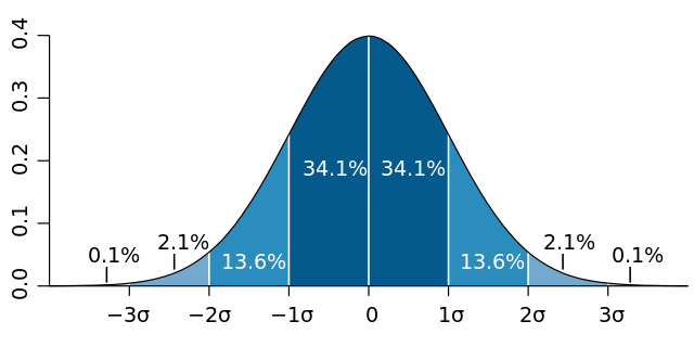
The normal distribution, or bell curve, describes the randomness of measurement. The mean, or average value, is at zero, while points fall farther and farther away with increasingly less likelihood.
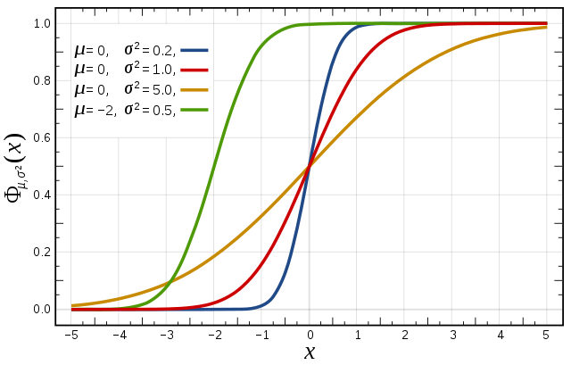
One way to get from a uniform random number to a normal random number is to use the uniform random number as the cumulative distribution function (CDF)↗, an index into “how far” the value is along the normal curve.
This is an approximation which is accurate to one decimal place:
where
- sgn is the signum or sign function.
To calculate an arbitrary power of a floating-point number, we require a few transcendental functions, in particular the natural logarithm and exponentiation of base . The following helper core contains relatively inefficient but clear implementations of standard numerical methods.
/gen/normal.hoon
Click to expand
!:=<|= n=@ud :: n is the number of values to return^- (list @rs)=/ values (rip 5 (~(lcg gen 20.220.524) n))=/ mask-clear 0b111.1111.1111.1111.1111.1111=/ mask-fill 0b11.1111.0000.0000.0000.0000.0000.0000=/ clears (turn values |=(a=@rs (dis mask-clear a)))=/ uniforms (turn clears |=(a=@ (sub:rs (mul:rs .2 (con mask-fill a)) .1.0)))(turn uniforms normal)|%++ factorial:: integer factorial, not gamma function|= x=@rs^- @rs=/ t=@rs .1|- ^- @rs?: |(=(x .1) (lth x .1)) t$(x (sub:rs x .1), t (mul:rs t x))++ absrs|= x=@rs ^- @rs?: (gth:rs x .0)x(sub:rs .0 x)++ exp|= x=@rs^- @rs=/ rtol .1e-5=/ p .1=/ po .-1=/ i .1|- ^- @rs?: (lth:rs (absrs (sub:rs po p)) rtol) p$(i (add:rs i .1), p (add:rs p (div:rs (pow-n x i) (factorial i))), po p)++ pow-n:: restricted power, based on integers only|= [x=@rs n=@rs]^- @rs?: =(n .0) .1=/ p x|- ^- @rs?: (lth:rs n .2) p$(n (sub:rs n .1), p (mul:rs p x))++ ln:: natural logarithm, z > 0|= z=@rs^- @rs=/ rtol .1e-5=/ p .0=/ po .-1=/ i .0|- ^- @rs?: (lth:rs (absrs (sub:rs po p)) rtol)(mul:rs (div:rs (mul:rs .2 (sub:rs z .1)) (add:rs z .1)) p)=/ term1 (div:rs .1 (add:rs .1 (mul:rs .2 i)))=/ term2 (mul:rs (sub:rs z .1) (sub:rs z .1))=/ term3 (mul:rs (add:rs z .1) (add:rs z .1))=/ term (mul:rs term1 (pow-n (div:rs term2 term3) i))$(i (add:rs i .1), p (add:rs p term), po p)++ powrs:: general power, based on logarithms:: x^n = exp(n ln x)|= [x=@rs n=@rs](exp (mul:rs n (ln x)))++ normal|= u=@rs(div:rs (sub:rs (powrs u .0.135) (powrs (sub:rs .1 u) .0.135)) .0.1975)++ gen|_ [z=@ud]++ lcg|= n=@ud :: n is the number of bits to return=/ a 742.938.285 :: a is the multiplier=/ e 31 :: e is the exponent=/ m (sub (pow 2 e) 1) :: modulus=/ index 0=/ accum *@ub|- ^- @ub?: =(index n) accum%= $index +(index)z (mod (mul a z) m)accum (cat 5 z accum)==----
Exercise: Upgrade the normal RNG
A more complicated formula uses several constants to improve the accuracy significantly:
where
- sgn is the signum or sign function;
- is ; and
- the constants are:
- Implement this formula in Hoon to produce normally-distributed random numbers.
- How would you implement other random number generators?
Hashing
A hash function↗ is a tool which can take any input data and produce a fixed-length value that corresponds to it. Hashes can be used for many purposes:
- Encryption. A cryptographic hash function↗ leans into the one-way nature of a hash calculation to produce a fast, practically-irreversible hash of a message. They are foundational to modern cryptography.
- Attestation or preregistration. If you wish to demonstrate that you produced a particular message at a later time (including a hypothesis or prediction), or that you solved a particular problem, hashing the text of the solution and posting the hash publicly allows you to verifiably timestamp your work.
- Integrity verification. By comparing the hash of data to its expected hash, you can verify that two copies of data are equivalent (such as a downloaded executable file). The MD5↗ hash algorithm is frequently used for this purpose as
md5sum. - Data lookup. Hash tables↗ are one way to implement a key→value mapping, such as the functionality offered by Hoon's ++map.
Theoretically, since the number of fixed-length hashes are finite, an infinite number of possible programs can yield any given hash. This is called a hash collision, but for many practical purposes such a collision is extremely unlikely.
Hoon Operations
The Hoon standard library supports fast insecure hashing with ++mug, which accepts any noun and produces an atom of the hash.
> `@ux`(mug 1)0x715c.2a60> `@ux`(mug 2)0x718b.9468> `@ux`(mug 3)0x72a8.ef1a> `@ux`(mug 1.000.000)0x5145.9d7d> `@ux`(mug .)0x6c91.8422
++mug operates on the raw form of the noun however, without Hoon-specific metadata like aura:
> (mug 0x5)721.923.263> (mug 5)721.923.263
Hoon also includes SHA-256 and SHA-512↗ tooling. (++og, the random number generator, is based on SHA-256 hashing.)
++shax produces a hashed atom of 256 bits from any atom.
69.779.012.276.202.546.540.741.613.998.220.636.891.790.827.476.075.440.677.599.814.057.037.833.368.907> `@ux`(shax 1)0x9a45.8577.3ce2.ccd7.a585.c331.d60a.60d1.e3b7.d28c.bb2e.de3b.c554.4534.2f12.f54b> `@ux`(shax 2)0x86d9.5764.98ea.764b.4924.3efe.b05d.f625.0104.38c6.a55d.5b57.8de4.ff00.c9b4.c1db> `@ux`(shax 3)0xc529.ffad.9a5a.b611.62b1.1d61.6b63.9e00.586b.a846.746a.197d.4daf.78b9.08ed.4f08> `@ux`(shax 1.000.000)0x84a4.929b.1d69.708e.d4b7.0fb8.ca97.cc85.c4a6.1aae.4596.f753.d0d2.6357.e7b9.eb0f++shaz produces a hashed atom of 512 bits from any atom.
> (shaz 1)3.031.947.054.025.992.811.210.838.487.475.158.569.967.793.095.050.169.760.709.406.427.393.828.309.497.273.121.275.530.382.185.415.047.474.588.395.933.812.689.047.905.034.106.140.802.678.745.778.695.328.891> `@ux`(shaz 1)0x39e3.d936.c6e3.1eaa.c08f.cfcf.e7bb.4434.60c6.1c0b.d5b7.4408.c8bc.c35a.6b8d.6f57.00bd.cdde.aa4b.466a.e65f.8fb6.7f67.ca62.dc34.149e.1d44.d213.ddfb.c136.68b6.547b> `@ux`(shaz 2)0xcadc.698f.ca01.cf29.35f7.6027.8554.b4e6.1f35.4539.75a5.bb45.3890.0315.9bc8.485b.7018.dd81.52d9.cc23.b6e9.dd91.b107.380b.9d14.ddbf.9cc0.37ee.53a8.57b6.c948.b8fa> `@ux`(shaz 3)0x4ba.a6ba.4a01.12e6.248b.5e89.9389.4786.aced.1a59.136b.78c6.7076.eb90.2221.d7a5.453a.56d1.446d.17d1.33cd.b468.f798.eb6b.dcee.f071.7040.7a2f.aa94.df7d.81f5.5be4> `@ux`(shaz 1.000.000)0x4c13.ef8b.09cf.6e59.05c4.f203.71a4.9cec.3432.ba26.0174.f964.48f1.5475.b2dd.2c59.98c2.017c.9c03.cbea.9d5f.591b.ff23.bbff.b0ae.9c67.a4a9.dd8d.748a.8e14.c006.cbcc
Exercise: Produce a secure password tool
- Produce a basic secure password tool. It should accept a password, salt it (add a predetermined value to the password), and hash it. That hash is then compared to a reference hash to determine whether or not the password is correct.